Confusion Matrix: A Way To Choose An Effective Threshold Value:
A confusion matrix also known as error matrix is a predictor of model performance on a classification problem. The number of correct and incorrect predictions is summarized with count values and broken down by each class. This lie at the core of the confusion matrix.
The confusion matrix shows the ways in which your classification model is confused when it makes predictions on observations, it helps us to measure the type of error our model is making while classifying the observation into different classes.
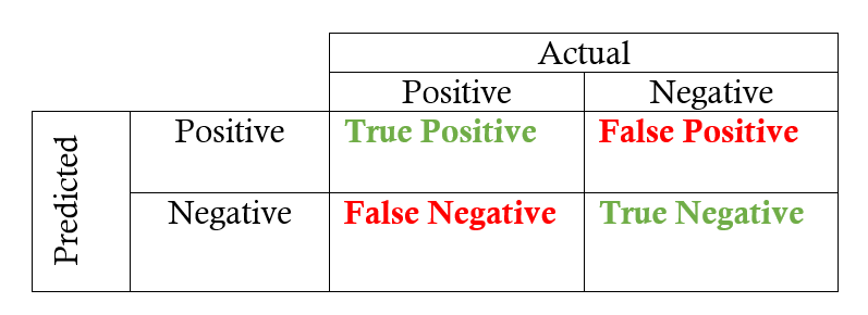
Key Parts Of Confusion Matrix:
- True Positive (TP): This refers to the cases in which we predicted “YES” and our prediction was actually TRUE(Eg. Patient is actually having diabetes and you predicted it to be True)
- True Negative (TN): This refers to the cases in which we predicted “NO” and our prediction was actually TRUE(Eg. Patient is not having diabetes and you predicted the same. )
- False Positive (FP): This refers to the cases in which we predicted “YES”, but our prediction turned out FALSE (Patient was not having diabetes, but our model predicted that s/he is diabetic)
- False Negative (FN): This refers to the cases in which we predicted “NO” but our prediction turned out FALSE
Key Learning Metrics From Confusion Matrix:
Confusion matrix helps us learn following metrics, helping us to measure logistic model performance.
Accuracy:
It answers:
Overall, how often is the classifier correct?
Accuracy = (TP+TN)/total No of Classified Item = (TP+TN)/ (TP+TN+FP+FN)
Precision:
It answers:
When it predicts yes, how often is it correct?
Precision is usually used when the goal is to limit the number of false positives(FP). For example, with the spam, filtering algorithm, where our aim is to minimize the number of reals emails that are classified as spam.
Precision = TP/ (TP+FP)
Recall:
It answers:
When it is actually the positive result, how often does it predict correctly?
It is calculated as,
Recall = TP/ (TP+FN), also known as sensitivity.
f1-score:
It is just the harmonic mean of precision and recall:
It is calculated as,
f1-score = 2*((precision*recall)/(precision+recall))
So when you need to take both precision and recall into account this f1 score is a useful metric to measure. If you try to only optimize recall, your algorithm will predict most examples to belong to the positive class, but that will result in many false positives and, hence, low precision. Also, if you try to optimize precision, your model will predict very few examples as positive results (the ones which highest probability), but recall will be very low. So it can be insightful to balance out and consider both and see the result.
AUC Area Under The Curve:
One more useful metric to evaluate and compare predictive models is the ROC curve.
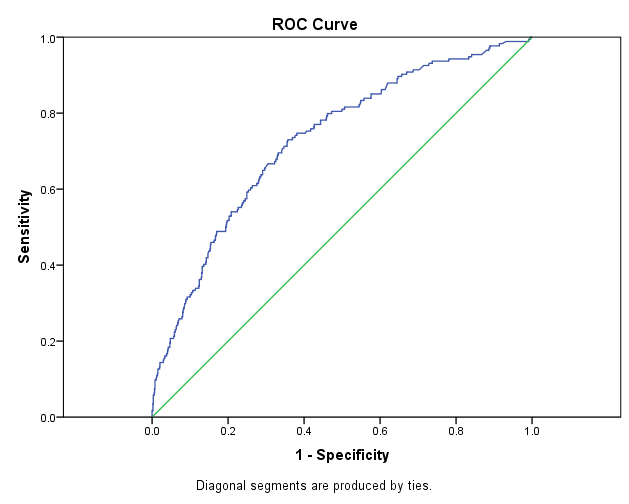
In statistics, a Receiver Operating Characteristic (ROC), or ROC curve, is a graphical plot that illustrates the performance of a binary classifier system as its discrimination threshold is varied. The curve is created by plotting the true positive rate (sensitivity) against the false positive rate (1 — specificity) at various threshold settings.
ROC curves are a nice way to see how any predictive model can distinguish between the true positives and negatives. The ROC curve plots out the sensitivity and specificity for every possible decision rule cutoff between 0 and 1 for a model.
Where,
Specificity or True Negative Rate = TN/(TN+FP)
Sensitivity or True Positive Rate= TP/(TP+FN)
So FPR, False Positive Rate = 1–Specificity
Intuition behind ROC curve is:
That the model which predicts at chance will have an ROC curve that looks like the diagonal green line(as shown above in the fig). That is not a discriminating model. The further the curve is from the diagonal line, the better the model is at discriminating between positives and negatives in general.